Example: (nonlinear) IV causal inference (no invalid IVs)
Below is an example that demonstrates the usage of
ts_twasinnl_causal.
Simulate Data
library:
nl_causal.base.simTwo Stage Datasets: two independent datasets, 2SLS and 2SIR require different types of datasets:
For 2SLS:
Stage 1. LD matrix (
np.dot(Z1.T, Z1)) + XZ_sum (np.dot(Z1.T, X1))Stage 2. ZY_sum (GWAS summary) (
np.dot(Z2.T, y2))
For 2SIR:
Stage 1. invidual-level data
Z1andX1Stage 2. ZY_sum (GWAS summary) (
np.dot(Z2.T, y2))
Remarks: In terms of data, the advantage of 2SLS is merely requiring summary statistics of XZ and YZ in both Stages 1 and 2.
[1]:
## import libraries
import numpy as np
from nl_causal.base import sim
from sklearn.preprocessing import StandardScaler
from sklearn.model_selection import train_test_split

## simulate a dataset
np.random.seed(0)
n, p = 3000, 20
beta0 = 0.10
theta0 = np.ones(p) / np.sqrt(p)
Z, X, y, phi = sim(n, p, theta0, beta0, case='log', feat='normal')
## generate two-stage dataset
Z1, Z2, X1, X2, y1, y2 = train_test_split(Z, X, y, test_size=0.5, random_state=42)
n1, n2 = len(Z1), len(Z2)
LD_Z1, cov_ZX1 = np.dot(Z1.T, Z1), np.dot(Z1.T, X1)
LD_Z2, cov_ZY2 = np.dot(Z2.T, Z2), np.dot(Z2.T, y2)
╔═════════════════════════════════════╗
║ True Model                          ║
║ ----------                          ║
║ ψ(x) = z^T θ + ω;                   ║
║ y = β ψ(x) + z^T α + ε.             ║
║ ---                                 ║
║ β: causal effect from x to y.       ║
║ ψ(x): causal link among (z, x, y).  ║
║ ---                                 ║
║ True β : 0.100                      ║
║ True ψ(x) : log                     ║
╚═════════════════════════════════════╝
Models
library:
nl_causal.ts_models._2SLSandnl_causal.ts_models._2SIRsparse regression:
sparse_reg=None: assume all IVs are valid.specify a sparse regression method from
sparse_regto detect invalid IVs, such asSCAD.
Remarks. 2SIR circumvents the linearity assumption in the standard 2SLS, and includes 2SLS as a special case.
[2]:
from nl_causal.ts_models import _2SLS, _2SIR
[3]:
## 2SLS
LS = _2SLS(sparse_reg=None)
## Stage-1 fit theta
LS.fit_theta(LD_Z1, cov_ZX1)
## Stage-2 fit beta
LS.fit_beta(LD_Z2, cov_ZY2, n2)
## produce p_value and CI for beta
LS.test_effect(n2, LD_Z2, cov_ZY2)
LS.CI_beta(n1, n2, Z1, X1, LD_Z2, cov_ZY2)
LS.summary()
╔════════════════════════════════════════════╗
║ 2SLS                                       ║
║ ----                                       ║
║ x = z^T θ + ω;                             ║
║ y = β x + z^T α + ε.                       ║
║ ---                                        ║
║ β: causal effect from x to y.              ║
║ ---                                        ║
║ Est β (CI): 0.040 (CI: [-0.1638  0.2433])  ║
║ p-value: 0.2968, -log10(p): 0.5275         ║
╚════════════════════════════════════════════╝
[4]:
## 2SIR
SIR = _2SIR(sparse_reg=None)
## Stage-1 fit theta
SIR.fit_theta(Z1, X1)
## Stage-2 fit beta
SIR.fit_beta(LD_Z2, cov_ZY2, n2)
## generate CI for beta
SIR.test_effect(n2, LD_Z2, cov_ZY2)
SIR.CI_beta(n1, n2, Z1, X1, LD_Z2, cov_ZY2)
SIR.summary()
╔══════════════════════════════════════════╗
║ 2SIR                                     ║
║ ----                                     ║
║ ψ(x) = z^T θ + ω;                        ║
║ y = β ψ(x) + z^T α + ε.                  ║
║ ---                                      ║
║ β: causal effect from x to y.            ║
║ ---                                      ║
║ Est β (CI): 0.080 (CI: [0.0079 0.1522])  ║
║ p-value: 0.0317, -log10(p): 1.4994       ║
╚══════════════════════════════════════════╝
Results
In the simulated data, the true causal effect is beta0 = 0.10.
2SLS provides wrong p-values and CIs, and fails to reject the null hypothesis that
H0: beta = 0.2SIR provides a valid CI and reject the null hypothesis.
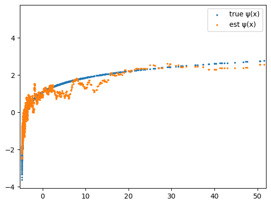
Estimation the causal link ψ(x)
This is only feasible for 2SIR.
[5]:
from sklearn.neighbors import KNeighborsRegressor

## fit the causal link
SIR.cond_mean=KNeighborsRegressor(n_neighbors=20)
SIR.fit_link(Z1=Z1, X1=X1)
# evalue ψ(x) based on the estimated causal link
est_phi = SIR.link(X[:,np.newaxis])
[6]:
import matplotlib.pyplot as plt

plt.xlim(1.1*np.quantile(X,.01), 1.1*np.quantile(X,.99))
plt.scatter(X, phi, s=2.5, label='true ψ(x)')
plt.scatter(X, est_phi, s=2.5, label='est ψ(x)')
plt.legend()
plt.show()