Example: (nonlinear) IV causal inference (with invalid IVs)
Below is an example that demonstrates the usage of
ts_twasinnl_causal.
Simulate Data
library:
nl_causal.base.simTwo Stage Datasets: two independent datasets, 2SLS and 2SIR require different types of datasets:
For 2SLS:
Stage 1. LD matrix (
np.dot(Z1.T, Z1)) + XZ_sum (np.dot(Z1.T, X1))Stage 2. ZY_sum (GWAS summary) (
np.dot(Z2.T, y2))
For 2SIR:
Stage 1. invidual-level data
Z1andX1Stage 2. ZY_sum (GWAS summary) (
np.dot(Z2.T, y2))
Remarks: In terms of data, the advantage of 2SLS is merely requiring summary statistics of XZ and YZ in both Stages 1 and 2.
[1]:
## import libraries
import numpy as np
from nl_causal.base import sim
from sklearn.preprocessing import StandardScaler
from sklearn.model_selection import train_test_split

## simulate a dataset
np.random.seed(1)
n, p = 2000, 20
beta0 = 0.10
theta0 = np.ones(p) / np.sqrt(p)
## simulate invalid IVs
alpha0 = np.zeros(p)
alpha0[:5] = 1.

Z, X, y, phi = sim(n, p, theta0, beta0, alpha0=alpha0, case='quad', feat='cate')

## generate two-stage dataset
Z1, Z2, X1, X2, y1, y2 = train_test_split(Z, X, y, test_size=0.5, random_state=42)
n1, n2 = len(Z1), len(Z2)
LD_Z1, cov_ZX1 = np.dot(Z1.T, Z1), np.dot(Z1.T, X1)
LD_Z2, cov_ZY2 = np.dot(Z2.T, Z2), np.dot(Z2.T, y2)
╔═════════════════════════════════════╗
║ True Model                          ║
║ ----------                          ║
║ ψ(x) = z^T θ + ω;                   ║
║ y = β ψ(x) + z^T α + ε.             ║
║ ---                                 ║
║ β: causal effect from x to y.       ║
║ ψ(x): causal link among (z, x, y).  ║
║ ---                                 ║
║ True β : 0.100                      ║
║ True ψ(x) : quad                    ║
╚═════════════════════════════════════╝
/home/ben/np/lib/python3.10/site-packages/nl_causal/base/sim_data.py:131: UserWarning: To better satisfy the <quad> causal link, both U and eps are currently configured as a uniform distribution.
  warnings.warn("To better satisfy the <quad> causal link, both U and eps are currently configured as a uniform distribution.")
Models
library:
nl_causal.ts_models._2SLSandnl_causal.ts_models._2SIRsparse regression:
sparse_reg=None: assume all IVs are valid.specify a sparse regression method from
sparse_regto detect invalid IVs, such asSCAD.
Remarks. 2SIR circumvents the linearity assumption in the standard 2SLS, and includes 2SLS as a special case.
[2]:
from nl_causal.ts_models import _2SLS, _2SIR
[3]:
## 2SLS

# specify a sparse regression model to detect invalid IVs
from nl_causal.sparse_reg import L0_IC
Ks = range(int(p/2))
reg_model = L0_IC(fit_intercept=False, alphas=10**np.arange(-1,3,.3),
                              Ks=Ks, max_iter=10000, refit=False, find_best=False)
LS = _2SLS(sparse_reg=reg_model)

## Stage-1 fit theta
LS.fit_theta(LD_Z1, cov_ZX1)
## Stage-2 fit beta
LS.fit_beta(LD_Z2, cov_ZY2, n2)
LS.selection_summary().head(5)
[3]:
| candidate_model | criteria | mse | |
|---|---|---|---|
| 0 | [0, 1, 2, 3, 4, 8, 9, 11, 15, 20] | -0.636229 | 0.493957 |
| 1 | [0, 1, 2, 3, 4, 9, 15, 20] | -0.633458 | 0.502218 |
| 2 | [0, 1, 2, 3, 4, 15, 20] | -0.633333 | 0.505763 |
| 3 | [0, 1, 2, 3, 4, 20] | -0.631729 | 0.510086 |
| 4 | [0, 1, 2, 3, 4, 8, 15, 20] | -0.631598 | 0.503154 |
[4]:
## produce p_value and CI for beta
LS.test_effect(n2, LD_Z2, cov_ZY2)
LS.CI_beta(n1, n2, Z1, X1, LD_Z2, cov_ZY2)
LS.summary()
╔═════════════════════════════════════════════╗
║ 2SLS                                        ║
║ ----                                        ║
║ x = z^T θ + ω;                              ║
║ y = β x + z^T α + ε.                        ║
║ ---                                         ║
║ β: causal effect from x to y.               ║
║ ---                                         ║
║ Est β (CI): -0.006 (CI: [-0.1942  0.1816])  ║
║ p-value: 0.9473, -log10(p): 0.0235          ║
╚═════════════════════════════════════════════╝
[5]:
## 2SIR

Ks = range(int(p/2))
reg_model = L0_IC(fit_intercept=False, alphas=10**np.arange(-1,3,.3),
                              Ks=Ks, max_iter=10000, refit=False, find_best=False)

SIR = _2SIR(sparse_reg=reg_model)
## Stage-1 fit theta
SIR.fit_theta(Z1, X1)
## Stage-2 fit beta
SIR.fit_beta(LD_Z2, cov_ZY2, n2)
SIR.selection_summary().head(5)
[5]:
| candidate_model | criteria | mse | |
|---|---|---|---|
| 0 | [0, 1, 2, 3, 4, 8, 11, 20] | -0.638966 | 0.499460 |
| 1 | [0, 1, 2, 3, 4, 8, 11, 15, 20] | -0.638859 | 0.496075 |
| 2 | [0, 1, 2, 3, 4, 8, 20] | -0.637662 | 0.503578 |
| 3 | [0, 1, 2, 3, 4, 20] | -0.637546 | 0.507128 |
| 4 | [0, 1, 2, 3, 4, 8, 11, 12, 20] | -0.635553 | 0.497717 |
[6]:
## generate CI for beta
SIR.test_effect(n2, LD_Z2, cov_ZY2)
SIR.CI_beta(n1, n2, Z1, X1, LD_Z2, cov_ZY2)
SIR.summary()
╔══════════════════════════════════════════╗
║ 2SIR                                     ║
║ ----                                     ║
║ ψ(x) = z^T θ + ω;                        ║
║ y = β ψ(x) + z^T α + ε.                  ║
║ ---                                      ║
║ β: causal effect from x to y.            ║
║ ---                                      ║
║ Est β (CI): 0.226 (CI: [0.0532 0.3978])  ║
║ p-value: 0.0129, -log10(p): 1.8900       ║
╚══════════════════════════════════════════╝
Inference Results
In the simulated data, the true causal effect is beta0 = 0.10.
2SLS provides wrong p-values and CIs, and fails to reject the null hypothesis that
H0: beta = 0.2SIR provides a valid CI and reject the null hypothesis.
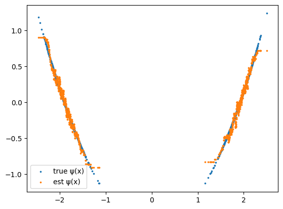
Estimation the causal link ψ(x)
This is only feasible for 2SIR.
[7]:
from sklearn.neighbors import KNeighborsRegressor

## fit the causal link
SIR.cond_mean=KNeighborsRegressor(n_neighbors=15)
SIR.fit_link(Z1=Z1, X1=X1)
# evalue ψ(x) based on the estimated causal link
est_phi = SIR.link(X[:,np.newaxis])
[8]:
import matplotlib.pyplot as plt

plt.xlim(1.1*min(X), 1.1*max(X))
plt.scatter(X, phi, s=2.5, label='true ψ(x)')
plt.scatter(X, est_phi, s=2.5, label='est ψ(x)')

plt.legend()
plt.show()